Robert Beazer

This document is a lab assignment using ArcGIS Model Builder that I prepared for students based on the topic of my Ph.D. research.

Abstract

The utility infrastructure in the United States is aging and increases in demand require the addition of new infrastructure.  Utility companies are exploring ways to augment this aging infrastructure and reduce its limitations.  As the heart of that process is a decision making process on where to find suitable locations to site a utility line.  ArcGIS Model Builder is suited well to assist in this process and answer the question of where best to construct this infrastructure.

Background

As a GIS professional you might be called upon to perform network analysis and create models that address the placement of utility lines.  The placement of utility lines is a hot button topic that makes modeling that placement extremely complex.  While in many cases a least cost path between two points would be a diagonal connecting line, engineering limitations and topography make the modeling of a least cost very difficult to overcome.   Additionally, when the court of public opinion is figured into the process, models of least cost can negate the feasible placement of a line as feelings of NIMBYism (Not In My Back Yard) or BANANAism (Build Absolutely Nothing Anywhere Near Anything) require rethinking the process. (Vajjhala and Fischbeck, 2006)  A GIS professional will be called upon to adjust inputs into the model to create paths to include many factors (Meehan, 2003) which makes the creation of an ArcGIS model paramount.  Additional layers, weights on those layers, and changing requirements can adjust the ultimate least cost path.  A standard model makes the creation of a path easier by automating the process so it can be used as many times as necessary to arrive at an acceptable path for all parties involved.  The purpose of this lab is to familiarize you with a few of the processes and requirements that might be used in the modeling of a least cost path for utility line placement.  You will not be asked to model social behaviors in this model, but will solely consider engineering aspects of the process. 

Limitations

            This lab simulates the placement of a high-voltage power line from to fictitious points in southeastern Idaho.  Although the start and end points for this lab are not real locations of substations or proposed substations, its purpose is to produce a model that is feasible for repetition on other projects where the points are real.  One major limitation in the creation of this lab was its setting in southeastern Idaho.  The requirements of avoiding rivers and major water bodies created an anomaly in this location as the Snake River bisects the area.  While the least cost path algorithm would still allow a path to cross the river at some point, the problem is that there is not really any control on where that happens.  Given this information, the addition of buffers around the cities that eliminated that requirement allowed more control over where the path would cross, but introduces another anomaly that may not be realistic—the placement of lines closer to cities which might not be the ideal or proper way to handle the problem.  Another limitation has to do with the way ArcGIS converts shapefiles into rasters.  When given a shapefile, ArcGIS forms the raster around the furthest most feature and the raster stops there.  So if there is a point in the middle of the area of interest, it forms a small raster there and no more.  This becomes a problem when doing an analysis such as this—the rasters have to be in common dimensions or the math, and ultimately the least cost path, will not work out correctly.  To account for this, additional features have to be created to match up the different layers and this creates anomalies that have to be accounted for.  In the reference map for this lab, there are four control points place at the edges of the area of interest that were created for the cities shapefile.  While these points did not have any bearing on this analysis, their buffers could skew results of another analysis.

Data Provided

            You will be provided with a geodatabase of the several feature classes you’ll need to complete this lab.  These classes include:

• Transportation data
  • Idaho_Roads12N is a feature class containing all of the roads in Idaho.  It was recent as of March 18, 2011 and was found at the InsideIdaho.org website.  For more current data you may download your own shapefile from the same site.  You will probably want to perform a definition query to select only the roads you’re interested in for this project.
• Hydrography data
  • Idaho_Lakes is a feature class that contains all of the lakes found in Idaho.  It was downloaded from the InsideIdaho.org website.
  • Idaho_Rivers is a feature class that shows the major rivers in Idaho.  It is from a national dataset which was then clipped to the boundaries of Idaho.
• Elevation data
  • ned30m_se is a raster dataset that contains elevation data for the tile that covers southeast Idaho.  This DEM was downloaded from the seamless server at the USGS website.
• Utility data
  • Proposed_Substations is a feature class that points out where the start and end points in the least cost path calculation should be.  These points do not represent actual or future substations.
• Other data
  • Idaho_Cities12N this feature class shows the major cities in southeastern Idaho.  It is from a national dataset which was clipped to the state of Idaho.  When considering the conversion of this point class, four points were added to the dataset to simulate four corners for the outline of the final raster dataset.

Model Builder Tasks

            The following Model Builder tools may be a part of your final model:

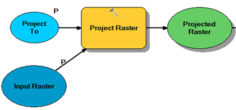
• Project Raster
• Buffer
• Erase
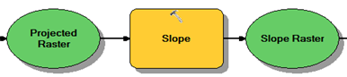
• Slope
• Polygon to Raster
• Raster Calculator
• Reclassify
• Cost Distance
• Cost Path
• Raster to Polyline

Lab Instructions

            Using ArcGIS 10 Model Builder and the data supplied, create a model that will site a power line considering the following criteria:

1. Lines should start at a proposed substation near Malad Idaho and terminate at a proposed substation at the Idaho/Montana border in southeastern Idaho.
2. Terrain grade should not exceed 30%.
3. Lines should be placed within two miles of a major highway or interstate.
4. Generally speaking, lines should not be placed within two miles of a major river or water body.
5. Cities have a ten mile radius that eliminates any constraint and allows a path to cross through it.

Hint: Use a uniform scale factor (perhaps 0 to 1) when using the raster calculator/reclassification tools to determine what locations would be suitable for siting a line.

For the purposes of this lab, assume that you are only creating a least cost path for the placement of a line.  Do not be concerned about the placement of individual towers.

Deliverables

            Once completed, submit your Model Builder process chart in its entirety and a map that demonstrates how you analyzed the included data and the results.  Your map should conform to generally accepted cartography standards and should include at minimum, a scale bar, north arrow, and legend.  Your deliverable should explain, in-depth, your Model Builder process and how it works.  Make sure to provide any equations you used in your calculations and feel free to share any challenges you faced as you completed the process.

            Use your Model Builder process to analyze the placement of another line of your choice.  This deliverable should use data you have compiled from reliable GIS data warehousing sources and must be outside of the extent of the data included with this lab.  Construct a map demonstrating the results of your model on this area using the same standards as outlined above.  Make sure to include the source information for any data you compile.

Reference Map

Possible Solution

 

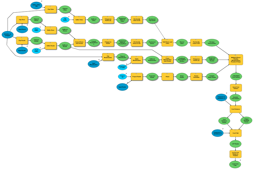
Step by Step:

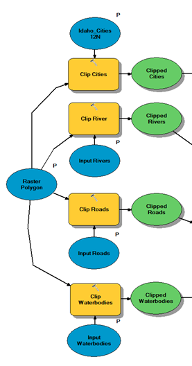
1. Clip all layers to the raster dataset.  This step limits each of the layers to the area of interest for the calculations and provides a cleaner final map.

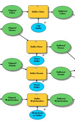
2. Perform the required buffers.  The requirements state that the lines need to be within two miles of a major road, cannot come within 2 miles of a major river or water body, and that there is a ten mile radius around cities that nullifies the above requirements.  This step performs each of these buffers.  Each buffer is parameterized to allow users to specify a buffer size.

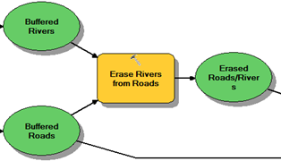
3. Erase rivers from roads.  Once the roads and rivers shapefiles are buffered it is necessary to exclude the areas where the rivers buffer coincides with the roads buffer.  The erase tool removes these areas so they will not be included in the final calculations as suitable areas for the line.

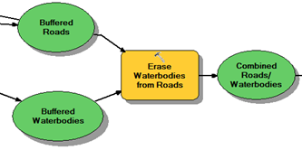
4. Erase water bodies from roads.  Similar to the roads and rivers buffers, the water body areas need to be removed from the roads buffer as not to be included in the final calculations.

5. Convert all buffer polygon layers to rasters.  Once all of the data layers are processed with their buffers and overlapping areas removed (rivers and water bodies), and added (cities), all layers need to be converted to a raster for future processing in a raster calculator.

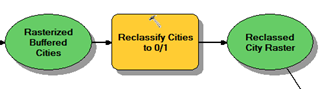
6. Reclassify cities raster.  In order to create the cities raster, four points were digitized, one on each of the four corners of the area of interest.  When a raster is created on points, it only creates a square around the existing points.  To make the raster similar in size to the other rasters in the series, these points had to be created.  This step isolates those points and reclassifies them to zero while the actual cities are reclassified to -101, which will be explained in a later step.

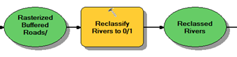
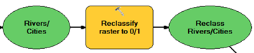
7. Reclassify buffered roads/rivers layer.  When this raster layer was created anything outside of the buffer was assigned a “no data” value.  This reclassification changes all the no data values to zero while the buffer’s value is changed to one.  This is necessary for the raster calculator later on as no data values propagate through each raster and will skew the results.

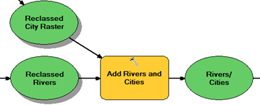
8. Add the cities and rivers buffers.  This step takes the cities and rivers buffers and, through a raster calculation, adds them together.  This is where the -101 reclassification becomes important from the previous step.  When the -101 is added to the rivers raster, the -101 value will eventually invert the buffer in the rivers layer satisfying the requirement that cities nullify the other requirements.

9. Reclassify the cities/rivers raster.  This step eliminates the -101 value from the previous step by assigning it a 1 while maintaining the zero areas as they are.  This results in a permitted/not permitted (0/1) raster and is prepared for the multiplication step which is to follow.

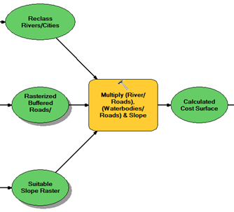
10. Calculate slope values for the area of interest.  This step is actually a combination of steps that calculate the slope in the area of interest and provides a 0/1 value raster when complete.  This will feed into the multiplication step that is to follow.

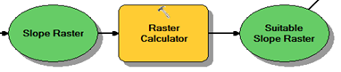
11. Multiply the three input layers together.  This is the crucial step.  Each of the prepared three layers, rivers/cities, slope, and water bodies/roads need to be multiplied together to create a preliminary cost surface.  This is where the 0/1 method works out.  Areas that are zero will multiply through and remain zero while areas that are permissible will retain the value of one.

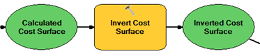
12. Invert the cost raster.  Now that there is a cost surface, it needs to be inverted to properly reflect a cost.  Since a zero value costs less than a one value to traverse, we want to reclassify the one values (areas that are permissible) to zero values and having less cost to traverse while reclassifying the zero values (areas not permissible) to one and hence a prohibitive cost to traverse.

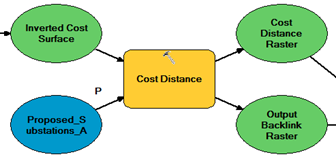
13. Perform the cost distance function.  This is the first of the least cost path functions.  This function calculates the bulk of the least cost path by creating two rasters that will feed into the cost path function which actually creates the least cost path.

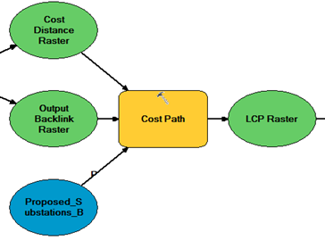
14. Perform the cost path function.  As mentioned in the previous step, this function actually creates the least cost path.  It takes the two cost rasters from the previous function and, along with the end point, creates the least cost path.

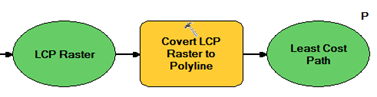
15. Convert Least Cost Path raster to a polyline shapefile.  This final step takes the least cost path raster and converts it to a polyline shapefile.  This makes the line more manageable as the line on the raster might be difficult to see.

References

Meehan, Bill. Case Studies in GIS: Empowering Electric and Gas Utilities with GIS. Redlands, California: ESRI Press, 2007.  Print.

Schmidt, Andrew J.  “Implementing a GIS Methodology for Siting High Voltage Electric Transmission Lines.”  Papers in Resource Analysis Volume 11.  Winona, Minnesota: Saint Mary’s University of Minnesota University Central Services Press, 2009.  Accessed 05 July 2010.  Web.

Vajjhala, Shalini P. and Paul S. Fischbeck.  “Quantifying Siting Difficulty: A Case Study of U.S. Transmission Line Siting.” Discussion Paper for Resources For the Future.  Accessed 24 June 2010.  Web. <url: www.rff.org/rff/documents/Rff-DP-06-03.pdf>